Introduction
This is a blog post to expand on a talk I gave at the Manchester R Users Group on 21st February 2017. In it I give a brief overview of the tidyverse and its core concepts, before going on to discuss how the same concepts can be applied to bioinformatics analysis using Bioconductor classes and packages.
What is the tidyverse?
The tidyverse is a suite of tools primarily developed by Hadley Wickham and collaborators at RStudio. The suite of packages can be conveniently installed as follows:
install.packages('tidyverse')There are many talks and resources that go into much greater depth than I do here including:
- Managing many models talk on YouTube by Hadley Wickham
- R for Data Science book and website
- Recorded tutorials and presentations from RStudio::conf 2017
- Webinars on RStudio website
- DataCamp courses on dplyr and the tidyverse
Key concepts in the tidyverse
Tidy data
They key concept of the tidyverse is that of tidy data. If you’re from a database background then think of this as normalised data. For example, the table below is NOT tidy data since the year variable is encoded as a column name:
library(tidyverse)
table4a
## # A tibble: 3 x 3
## country `1999` `2000`
## * <chr> <int> <int>
## 1 Afghanistan 745 2666
## 2 Brazil 37737 80488
## 3 China 212258 213766To turn this into tidy data with one observation per row, we can use the tidyr package:
df <- gather(table4a, year, cases, -country)
df
## # A tibble: 6 x 3
## country year cases
## <chr> <chr> <int>
## 1 Afghanistan 1999 745
## 2 Brazil 1999 37737
## 3 China 1999 212258
## 4 Afghanistan 2000 2666
## 5 Brazil 2000 80488
## 6 China 2000 213766Tibbles
Tibbles are an alternative to the data frame. The key differences are:
- Subsetting a tibble will always produce another tibble.
- A tibble will only print to screen - no more pages of output…
dplyr::filter(df, cases == 'Nigeria')## # A tibble: 0 x 3
## # ... with 3 variables: country <chr>, year <chr>, cases <int>dplyr::select(df, country)## # A tibble: 6 x 1
## country
## <chr>
## 1 Afghanistan
## 2 Brazil
## 3 China
## 4 Afghanistan
## 5 Brazil
## 6 Chinalibrary(gapminder)## Warning: package 'gapminder' was built under R version 3.4.2gapminder## # A tibble: 1,704 x 6
## country continent year lifeExp pop gdpPercap
## <fctr> <fctr> <int> <dbl> <int> <dbl>
## 1 Afghanistan Asia 1952 28.801 8425333 779.4453
## 2 Afghanistan Asia 1957 30.332 9240934 820.8530
## 3 Afghanistan Asia 1962 31.997 10267083 853.1007
## 4 Afghanistan Asia 1967 34.020 11537966 836.1971
## 5 Afghanistan Asia 1972 36.088 13079460 739.9811
## 6 Afghanistan Asia 1977 38.438 14880372 786.1134
## 7 Afghanistan Asia 1982 39.854 12881816 978.0114
## 8 Afghanistan Asia 1987 40.822 13867957 852.3959
## 9 Afghanistan Asia 1992 41.674 16317921 649.3414
## 10 Afghanistan Asia 1997 41.763 22227415 635.3414
## # ... with 1,694 more rowsdplyr and the pipe - %>%
The dplyr package provides an intuitive way of manipulating data frames that will come naturally to people from a database background who are used to SQL. Furthermore, the pipe operator allows function calls to be strung together sequentially rather than nested which improves readability. For example, the statements below:
# base r
gapminder[gapminder$country=='China', c('country', 'continent', 'year', 'lifeExp')]

# dplyr
dplyr::select(dplyr::filter(gapminder, country=='China'), country, continent, year, lifeExp)
Give the same output as this:
# pipe and dplyr
gapminder %>%
    dplyr::filter(country=='China') %>%
    dplyr::select(country, continent, year, lifeExp)
## # A tibble: 12 x 4
## country continent year lifeExp
## <fctr> <fctr> <int> <dbl>
## 1 China Asia 1952 44.00000
## 2 China Asia 1957 50.54896
## 3 China Asia 1962 44.50136
## 4 China Asia 1967 58.38112
## 5 China Asia 1972 63.11888
## 6 China Asia 1977 63.96736
## 7 China Asia 1982 65.52500
## 8 China Asia 1987 67.27400
## 9 China Asia 1992 68.69000
## 10 China Asia 1997 70.42600
## 11 China Asia 2002 72.02800
## 12 China Asia 2007 72.96100The RStudio Data Wrangling cheatsheet provides a useful resource for getting to know dplyr.
purrr and its map function
The purrr package provides a number of functions to make R more consistent and programming friendly than the equivalent base R functions. At first it’s map function seems like a reimplementation of apply:
map(c(4, 9, 16), sqrt)## [[1]]
## [1] 2
##
## [[2]]
## [1] 3
##
## [[3]]
## [1] 4But map will always return a list, and there are other members of the map_ family which will always return a certain data type:
map_dbl(c(4, 9, 16), sqrt)## [1] 2 3 4map_chr(c(4, 9, 16), sqrt)## [1] "2.000000" "3.000000" "4.000000"List-cols in data frames
List-cols are a powerful concept that underpin the later part of this tutorial. If data frames are explained as a way to keep character and number vectors together, then list-cols in tibbles takes this a step further and allow lists of any object to be kept together. For example, we can create nested data frames where we have a data frame within a data frame:
gm_nest <- gapminder %>% group_by(country, continent) %>% nest()
gm_nest
## # A tibble: 142 x 3
## country continent data
## <fctr> <fctr> <list>
## 1 Afghanistan Asia <tibble [12 x 4]>
## 2 Albania Europe <tibble [12 x 4]>
## 3 Algeria Africa <tibble [12 x 4]>
## 4 Angola Africa <tibble [12 x 4]>
## 5 Argentina Americas <tibble [12 x 4]>
## 6 Australia Oceania <tibble [12 x 4]>
## 7 Austria Europe <tibble [12 x 4]>
## 8 Bahrain Asia <tibble [12 x 4]>
## 9 Bangladesh Asia <tibble [12 x 4]>
## 10 Belgium Europe <tibble [12 x 4]>
## # ... with 132 more rowsSince the data column is a list column (list-col) we can access it as we would expect from a list. For example, to get the data for the second row, Albania:
gm_nest$data[[2]]## # A tibble: 12 x 4
## year lifeExp pop gdpPercap
## <int> <dbl> <int> <dbl>
## 1 1952 55.230 1282697 1601.056
## 2 1957 59.280 1476505 1942.284
## 3 1962 64.820 1728137 2312.889
## 4 1967 66.220 1984060 2760.197
## 5 1972 67.690 2263554 3313.422
## 6 1977 68.930 2509048 3533.004
## 7 1982 70.420 2780097 3630.881
## 8 1987 72.000 3075321 3738.933
## 9 1992 71.581 3326498 2497.438
## 10 1997 72.950 3428038 3193.055
## 11 2002 75.651 3508512 4604.212
## 12 2007 76.423 3600523 5937.030Using map to manipulate list-cols
Since this list column is just a list, we can use map to count the number of rows in each data frame in the list:
map_dbl(gm_nest[1:10,]$data, nrow)## [1] 12 12 12 12 12 12 12 12 12 12Rather than providing a ready to use function we can also define our own:
map_dbl(gm_nest[1:10,]$data, function(x) nrow(x))## [1] 12 12 12 12 12 12 12 12 12 12There is also a shorthand formula syntax for this where the period . represents the element of the list that is being processed:
map_dbl(gm_nest[1:10,]$data, ~nrow(.))## [1] 12 12 12 12 12 12 12 12 12 12Defining our own function allows us to reach into the data frame and perform an operation, such as summarise one of the columns:
map_dbl(gm_nest[1:10,]$data, ~round(mean(.$lifeExp),1))## [1] 37.5 68.4 59.0 37.9 69.1 74.7 73.1 65.6 49.8 73.6Importantly we can also do this at the level of the parent tibble and store the output in the data frame:
gm_nest %>% mutate(avg_lifeExp=map_dbl(data, ~round(mean(.$lifeExp),1)))## # A tibble: 142 x 4
## country continent data avg_lifeExp
## <fctr> <fctr> <list> <dbl>
## 1 Afghanistan Asia <tibble [12 x 4]> 37.5
## 2 Albania Europe <tibble [12 x 4]> 68.4
## 3 Algeria Africa <tibble [12 x 4]> 59.0
## 4 Angola Africa <tibble [12 x 4]> 37.9
## 5 Argentina Americas <tibble [12 x 4]> 69.1
## 6 Australia Oceania <tibble [12 x 4]> 74.7
## 7 Austria Europe <tibble [12 x 4]> 73.1
## 8 Bahrain Asia <tibble [12 x 4]> 65.6
## 9 Bangladesh Asia <tibble [12 x 4]> 49.8
## 10 Belgium Europe <tibble [12 x 4]> 73.6
## # ... with 132 more rowsThe power of list-cols
We could have summarised the gapminder data entirely in dplyr without worrying about list-cols and nested data frames:
gapminder %>%
    group_by(country) %>%
    summarise(avg_lifeExp=round(mean(lifeExp),1))
## # A tibble: 142 x 2
## country avg_lifeExp
## <fctr> <dbl>
## 1 Afghanistan 37.5
## 2 Albania 68.4
## 3 Algeria 59.0
## 4 Angola 37.9
## 5 Argentina 69.1
## 6 Australia 74.7
## 7 Austria 73.1
## 8 Bahrain 65.6
## 9 Bangladesh 49.8
## 10 Belgium 73.6
## # ... with 132 more rowsHowever, by using map rather than map_dbl we can create new list-cols, which can contain lists of any object that we want. In the example below we create a plot for each country, then display the first plot for Afghanistan:
gm_plots <- gm_nest %>%
    mutate(plot=map(data, ~qplot(x=year, y=lifeExp, data=.)))
gm_plots
## # A tibble: 142 x 4
## country continent data plot
## <fctr> <fctr> <list> <list>
## 1 Afghanistan Asia <tibble [12 x 4]> <S3: gg>
## 2 Albania Europe <tibble [12 x 4]> <S3: gg>
## 3 Algeria Africa <tibble [12 x 4]> <S3: gg>
## 4 Angola Africa <tibble [12 x 4]> <S3: gg>
## 5 Argentina Americas <tibble [12 x 4]> <S3: gg>
## 6 Australia Oceania <tibble [12 x 4]> <S3: gg>
## 7 Austria Europe <tibble [12 x 4]> <S3: gg>
## 8 Bahrain Asia <tibble [12 x 4]> <S3: gg>
## 9 Bangladesh Asia <tibble [12 x 4]> <S3: gg>
## 10 Belgium Europe <tibble [12 x 4]> <S3: gg>
## # ... with 132 more rowsgm_plots$plot[[1]]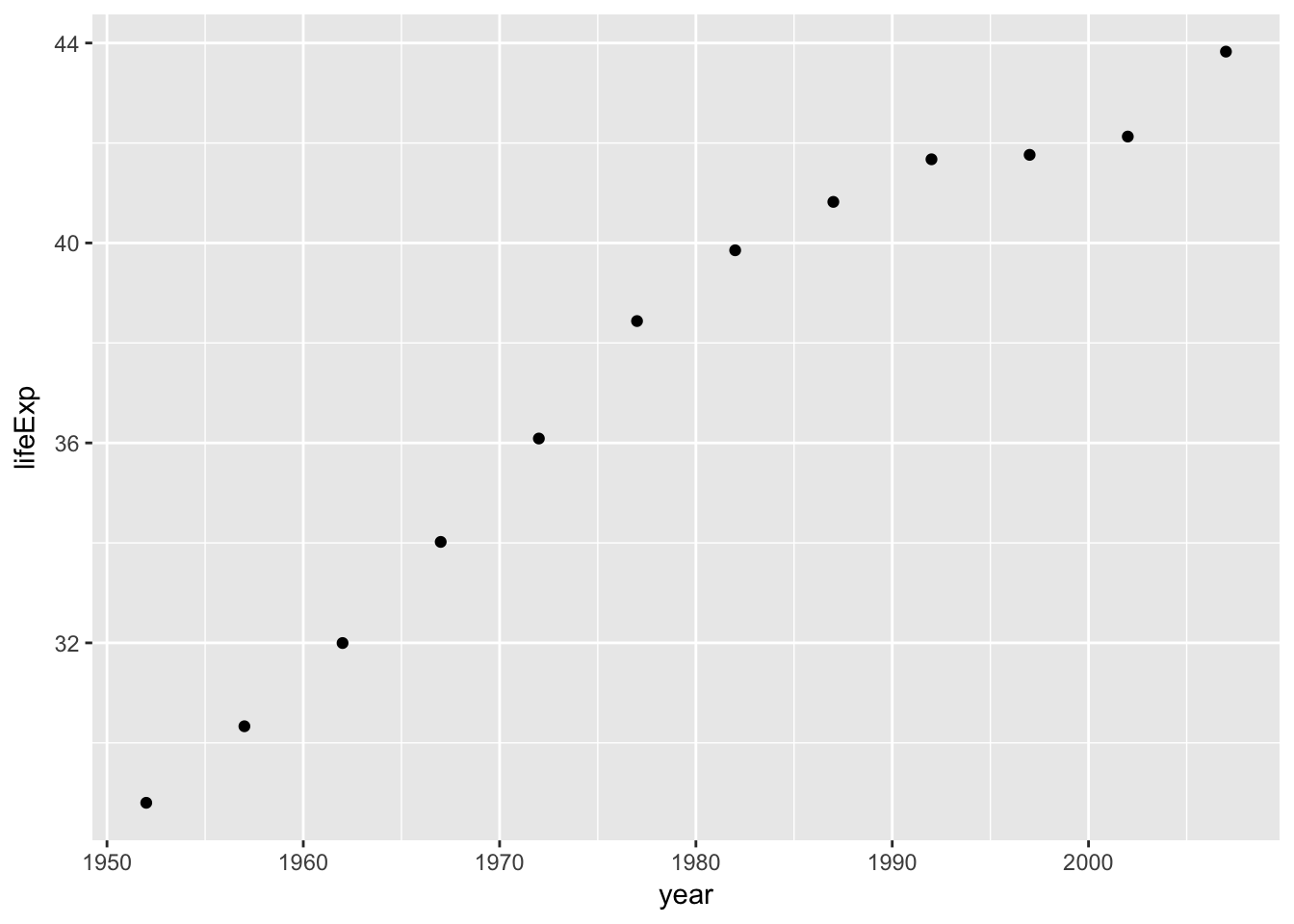
A complete example
In this example we combine the approaches described so far to:
- Nest the data
- Fit a linear regression model for each country
- Extract the slope and r2 value for each country
- Plot all countries together
gapminder_analysis <- gapminder %>%
    group_by(country, continent) %>%
    nest() %>%
    mutate(model=map(data, ~lm(lifeExp ~ year, data=.)),
           slope=map_dbl(model, ~coef(.)['year']),
           r2=map_dbl(model, ~broom::glance(.)$`r.squared`))
gapminder_analysis
## # A tibble: 142 x 6
## country continent data model slope r2
## <fctr> <fctr> <list> <list> <dbl> <dbl>
## 1 Afghanistan Asia <tibble [12 x 4]> <S3: lm> 0.2753287 0.9477123
## 2 Albania Europe <tibble [12 x 4]> <S3: lm> 0.3346832 0.9105778
## 3 Algeria Africa <tibble [12 x 4]> <S3: lm> 0.5692797 0.9851172
## 4 Angola Africa <tibble [12 x 4]> <S3: lm> 0.2093399 0.8878146
## 5 Argentina Americas <tibble [12 x 4]> <S3: lm> 0.2317084 0.9955681
## 6 Australia Oceania <tibble [12 x 4]> <S3: lm> 0.2277238 0.9796477
## 7 Austria Europe <tibble [12 x 4]> <S3: lm> 0.2419923 0.9921340
## 8 Bahrain Asia <tibble [12 x 4]> <S3: lm> 0.4675077 0.9667398
## 9 Bangladesh Asia <tibble [12 x 4]> <S3: lm> 0.4981308 0.9893609
## 10 Belgium Europe <tibble [12 x 4]> <S3: lm> 0.2090846 0.9945406
## # ... with 132 more rowsggplot(gapminder_analysis, aes(y=slope, colour=r2, x=continent)) +
geom_point(position=position_jitter(w=0.2)) +
theme_bw()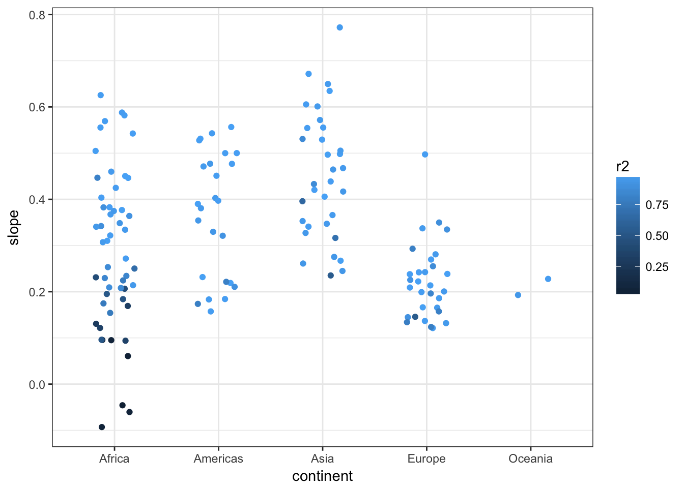
We can see that countries in Asia have has a faster increase in lifespan than those in Europe, whilst for Africa the picture is rather more mixed with some countries increasing and others staying the same or reducing and fitting more poorly to the linear regression model. Further analysis shows that the reasons for this include genocide and the HIV/AIDS epidemic.
This example demonstrates how powerful analyses can be carried out with very concise and non-repetitive code using tidyverse principles.
The tidyverse for Bioinformatics
What is Bioconductor?
Bioconductor is a suite of R packages and classes. This allows biological data to be analysed and stored in efficient and consistent ways. Analyses such as RNAseq analysis can also be controlled effectively using the list-cols framework.
A typical RNA-seq workflow
RNA-sequencing is carried out to quantitate the amount of a gene present in a set of samples. This can be done for all genes in the human genome simulatenously through the power of DNA sequencing. We then ask which genes are differentially expressed - ie are present in a different abundance in one set of samples (eg from a tumour) than another (eg normal). A typical RNA-seq experiment will have the following workflow:
- Align and count reads to form a SummarizedExperiment object
- Filter out genes with a low signal
- Specify a design formula to do the differential expression
- Specify a log2 fold change threshold to test for differentially expressed genes
- Plot the results
An RNA-seq analysis
First load the SummarizedExperiment object and explore it:
#adapted from https://f1000research.com/articles/4-1070/v2
library(airway)
library(DESeq2)
data(airway)
se <- airway
se
## class: RangedSummarizedExperiment
## dim: 64102 8
## metadata(1): ''
## assays(1): counts
## rownames(64102): ENSG00000000003 ENSG00000000005 ... LRG_98 LRG_99
## rowData names(0):
## colnames(8): SRR1039508 SRR1039509 ... SRR1039520 SRR1039521
## colData names(9): SampleName cell ... Sample BioSamplecolData(se)## DataFrame with 8 rows and 9 columns
## SampleName cell dex albut Run avgLength
## <factor> <factor> <factor> <factor> <factor> <integer>
## SRR1039508 GSM1275862 N61311 untrt untrt SRR1039508 126
## SRR1039509 GSM1275863 N61311 trt untrt SRR1039509 126
## SRR1039512 GSM1275866 N052611 untrt untrt SRR1039512 126
## SRR1039513 GSM1275867 N052611 trt untrt SRR1039513 87
## SRR1039516 GSM1275870 N080611 untrt untrt SRR1039516 120
## SRR1039517 GSM1275871 N080611 trt untrt SRR1039517 126
## SRR1039520 GSM1275874 N061011 untrt untrt SRR1039520 101
## SRR1039521 GSM1275875 N061011 trt untrt SRR1039521 98
## Experiment Sample BioSample
## <factor> <factor> <factor>
## SRR1039508 SRX384345 SRS508568 SAMN02422669
## SRR1039509 SRX384346 SRS508567 SAMN02422675
## SRR1039512 SRX384349 SRS508571 SAMN02422678
## SRR1039513 SRX384350 SRS508572 SAMN02422670
## SRR1039516 SRX384353 SRS508575 SAMN02422682
## SRR1039517 SRX384354 SRS508576 SAMN02422673
## SRR1039520 SRX384357 SRS508579 SAMN02422683
## SRR1039521 SRX384358 SRS508580 SAMN02422677colnames(assay(se))## [1] "SRR1039508" "SRR1039509" "SRR1039512" "SRR1039513" "SRR1039516"
## [6] "SRR1039517" "SRR1039520" "SRR1039521"rownames(assay(se))[1:10]## [1] "ENSG00000000003" "ENSG00000000005" "ENSG00000000419"
## [4] "ENSG00000000457" "ENSG00000000460" "ENSG00000000938"
## [7] "ENSG00000000971" "ENSG00000001036" "ENSG00000001084"
## [10] "ENSG00000001167"assay(se)[1:5,1:5]## SRR1039508 SRR1039509 SRR1039512 SRR1039513 SRR1039516
## ENSG00000000003 679 448 873 408 1138
## ENSG00000000005 0 0 0 0 0
## ENSG00000000419 467 515 621 365 587
## ENSG00000000457 260 211 263 164 245
## ENSG00000000460 60 55 40 35 78We can count up the number of reads per sample using the colSums function, or using purrr:
colSums(assay(se))## SRR1039508 SRR1039509 SRR1039512 SRR1039513 SRR1039516 SRR1039517
## 20637971 18809481 25348649 15163415 24448408 30818215
## SRR1039520 SRR1039521
## 19126151 21164133purrr::map_dbl(colnames(assay(se)), ~sum(assay(se)[,.]))## [1] 20637971 18809481 25348649 15163415 24448408 30818215 19126151 21164133We then create a DESeqDataSet object and set the design formula
dds <- DESeqDataSet(se, design = ~ cell + dex)Get rid of genes with few reads
dds <- dds[ rowSums(counts(dds)) > 1, ]Re-count the library size:
dds <- estimateSizeFactors(dds)Do a Principal Compnent Analysis to understand the data structure:
rld <- vst(dds, blind=FALSE)
pca_plot <- plotPCA(rld, intgroup = c("dex", "cell"))
pca_plot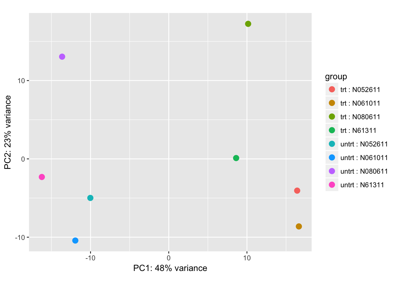
Do the differential expression analysis and extract the results:
dds <- DESeq(dds, quiet = TRUE)
res <- results(dds, lfcThreshold=0, tidy = TRUE) %>% tbl_df()
res
## # A tibble: 29,391 x 7
## row baseMean log2FoldChange lfcSE stat
## <chr> <dbl> <dbl> <dbl> <dbl>
## 1 ENSG00000000003 708.6021697 0.38125397 0.10065597 3.7876937
## 2 ENSG00000000419 520.2979006 -0.20681259 0.11222180 -1.8428915
## 3 ENSG00000000457 237.1630368 -0.03792034 0.14345322 -0.2643394
## 4 ENSG00000000460 57.9326331 0.08816367 0.28716771 0.3070111
## 5 ENSG00000000938 0.3180984 1.37822703 3.49987280 0.3937935
## 6 ENSG00000000971 5817.3528677 -0.42640216 0.08831006 -4.8284666
## 7 ENSG00000001036 1282.1063855 0.24107123 0.08871987 2.7172180
## 8 ENSG00000001084 609.8920919 0.04761687 0.16665615 0.2857192
## 9 ENSG00000001167 369.3428078 0.50036451 0.12088513 4.1391733
## 10 ENSG00000001460 183.2376742 0.12389881 0.17991227 0.6886624
## # ... with 29,381 more rows, and 2 more variables: pvalue <dbl>,
## # padj <dbl>Plot the results as an MA plot with abundance of the gene on the x-axis and fold change on the y-axis. Colour represents significance of the statistical test.
ma_plot <- ggplot(res, aes(log2(baseMean), log2FoldChange, colour=padj<0.1)) +
    geom_point(size=rel(0.5), aes(text=row)) + theme_bw()
## Warning: Ignoring unknown aesthetics: textma_plot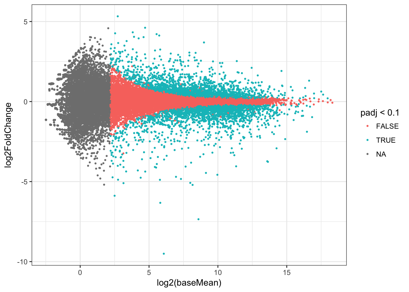
We can look at the top differentially expressed gene to see that there is indeed a difference between treated and untreated:
topGene <- res %>% dplyr::arrange(padj) %>%
    dplyr::slice(1) %>% dplyr::select(row) %>% unlist() %>% unname()
plotCounts(dds, gene=topGene, intgroup=c("dex"))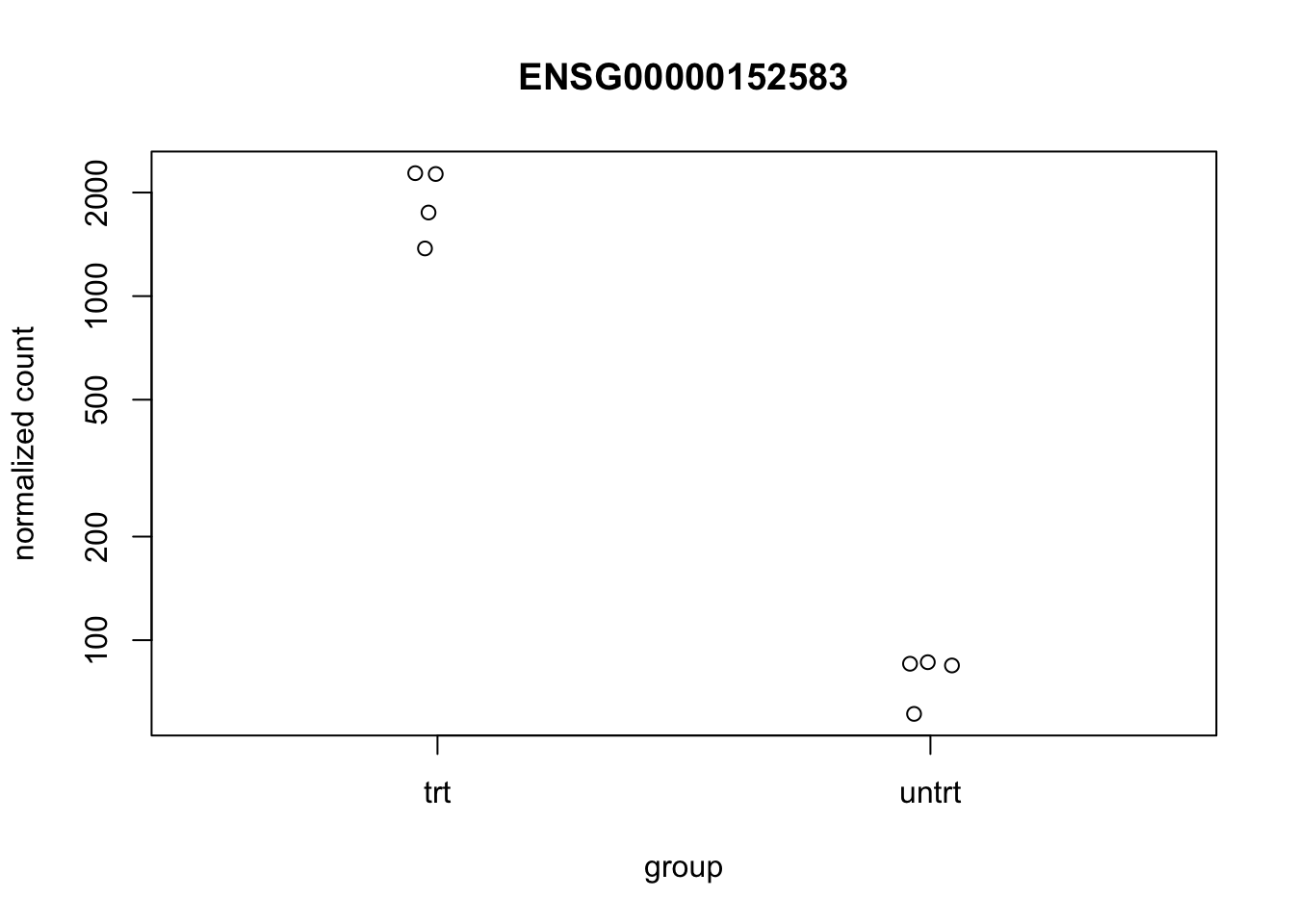
RNA-seq in the tidyverse
In the workflow there were a number of parameters that we might wish to vary:
- the design formula
- the log2 fold change threshold (
lfcThreshold) - the minimum read count
We can set up a control data frame using the tidyr::crossing function which contains 1 row per combination of parameters, and then add in the SummarizedExperiment object and a row number:
control_df <- tidyr::crossing(formula=c("~ cell + dex", "~ dex"),
                       lfcThreshold=c(0,1),
                       min_count=c(1,5))
control_df <- control_df %>% mutate(rn=row_number(),
                                    se=map(rn, ~se))
control_df
## # A tibble: 8 x 5
## formula lfcThreshold min_count rn
## <chr> <dbl> <dbl> <int>
## 1 ~ cell + dex 0 1 1
## 2 ~ cell + dex 0 5 2
## 3 ~ cell + dex 1 1 3
## 4 ~ cell + dex 1 5 4
## 5 ~ dex 0 1 5
## 6 ~ dex 0 5 6
## 7 ~ dex 1 1 7
## 8 ~ dex 1 5 8
## # ... with 1 more variables: se <list>Using map2 we can execute the DESeqDataSet function for each row taking the design formula and SummarizedExperiment object as inputs:
results_df <- control_df %>%
    mutate(dds=map2(se, formula, ~DESeqDataSet(.x, design=as.formula(.y))))
results_df
## # A tibble: 8 x 6
## formula lfcThreshold min_count rn
## <chr> <dbl> <dbl> <int>
## 1 ~ cell + dex 0 1 1
## 2 ~ cell + dex 0 5 2
## 3 ~ cell + dex 1 1 3
## 4 ~ cell + dex 1 5 4
## 5 ~ dex 0 1 5
## 6 ~ dex 0 5 6
## 7 ~ dex 1 1 7
## 8 ~ dex 1 5 8
## # ... with 2 more variables: se <list>, dds <list>At this point it is worth sanity checking that we have done what we wanted to do by comparing the input formula with that extracted from the DESeqDataSet:
results_df$formula## [1] "~ cell + dex" "~ cell + dex" "~ cell + dex" "~ cell + dex"
## [5] "~ dex" "~ dex" "~ dex" "~ dex"map_chr(results_df$dds, ~design(.) %>% as.character() %>% paste(collapse=' '))## [1] "~ cell + dex" "~ cell + dex" "~ cell + dex" "~ cell + dex"
## [5] "~ dex" "~ dex" "~ dex" "~ dex"Then finish off preparing the DESeqDataset object by removing genes below a certain read count:
results_df <- results_df %>%
    mutate(dds=map2(dds, min_count, ~.x[ rowSums(counts(.x)) > .y , ]),
           dds=map(dds, estimateSizeFactors))
And then doing the differential expression analysis itself and extracting the results:
results_df <- results_df %>%
    mutate(dds=map(dds, ~DESeq(., quiet=TRUE)),
           res=map2(dds, lfcThreshold, ~results(.x, lfcThreshold=.y, tidy = TRUE) %>% tbl_df()))
Viewing the results
At this point we can add a plot object to the mix like we did for the gapminder example. We define a plotting function to make the analysis more readable:
#define a plot function
my_plot <- function(df, pthresh) {
    ggplot(df, aes(log2(baseMean), log2FoldChange, colour=padj<pthresh)) +
        geom_point(size=rel(0.5)) +
        theme_bw()
}

#make the plots
plots_df <- results_df %>%
    mutate(ma_plot=map2(res, rn, ~my_plot(.x, 0.1) + ggtitle(.y)))
plots_df
## # A tibble: 8 x 8
## formula lfcThreshold min_count rn
## <chr> <dbl> <dbl> <int>
## 1 ~ cell + dex 0 1 1
## 2 ~ cell + dex 0 5 2
## 3 ~ cell + dex 1 1 3
## 4 ~ cell + dex 1 5 4
## 5 ~ dex 0 1 5
## 6 ~ dex 0 5 6
## 7 ~ dex 1 1 7
## 8 ~ dex 1 5 8
## # ... with 4 more variables: se <list>, dds <list>, res <list>,
## # ma_plot <list>We can then display the plots from the ma_plot list-col:
cowplot::plot_grid(plotlist=plots_df$ma_plot[1:4])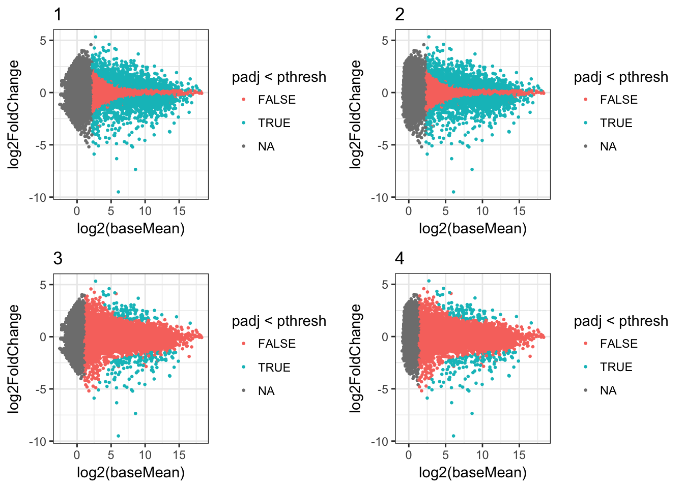
Or we can filter the data frame and just show some plots, for example those where the minimum read count was 1:
plots_df %>%
    dplyr::filter(min_count==1) %>%
    dplyr::select(ma_plot) %>%
    .$ma_plot %>%
    cowplot::plot_grid(plotlist=.)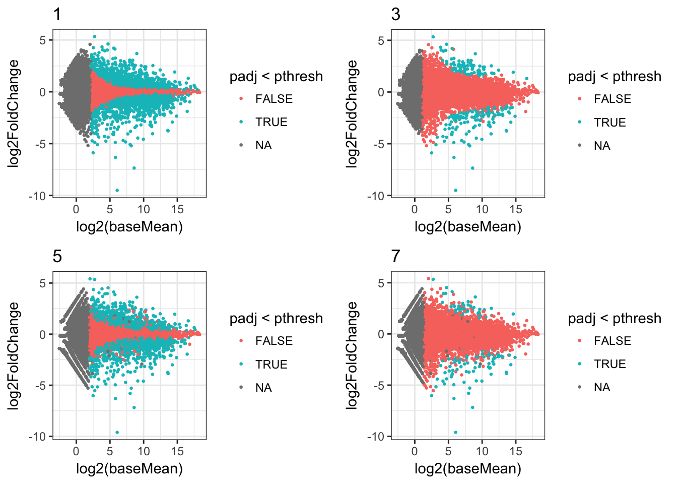
Limitations
Although the list-col approach provides useful framework for this type of analysis it does have some limitations:
- All of the data and results have to be held in the memory of one session.
- Can end up with multiple copies of data and very large data frames - models and plots will often contain the same data within the R object.
- Operations on a normal list can be easily parallelised using parallel::parLapply for example. This is more difficult using the list-col approach although one way is to split the tibble into a list of tibbles, and then parallelise across this.
- It can also be hard to wrap your brain around the necessary levels of abstraction!
Conclusion
Storing and manipulating objects in a data frame is a powerful and useful framework for an analysis since it keeps related things together and avoids code repetition and bloat. Analyses are parameterised which makes it very easy to add new values or change existing onces without copying and pasting big bits of code or having huge complicated functions. Although in this post it is applied to bioinformatics it could be applied to anything where work is done in specialised R object classes.
There is lots of work being done in the R community to extend these concepts, so keep an eye out for online presentations and tutorials!!