Introduction
In this example we do some very simple modelling using cancer cell line screening data and associated genetic data. The purpose of this example is to demonstrate how data can be extracted from PharmacoSet objects and then be used to develop linear models of dose response vs genetic features. However, there are uncertainties around IC50 estimation and cell line genetic feature classification (and meaning) which aren’t carried through into the modelling.
Get the data
PharmacoSet objects can be downloaded as follows (commented out for speed of rendering):
#ccle_pset <- downloadPSet('CCLE', saveDir='~/BigData/PSets/')
#gdsc_pset <- downloadPSet('GDSC', saveDir='~/BigData/PSets/')
And then loaded in the normal way:
load('~/BigData/PSets/GDSC.RData')Explore the PharmacoSet objects
Objects have a show method so calling the name of the object reveals lots of useful information about it.
GDSC## Name: GDSC
## Date Created: Wed Dec 30 10:44:21 2015
## Number of cell lines: 1124
## Number of drug compounds: 139
## RNA:
## Dim: 11833 789
## CNV:
## Dim: 24960 936
## Drug pertubation:
## Please look at pertNumber(pSet) to determine number of experiments for each drug-cell combination.
## Drug sensitivity:
## Number of Experiments: 79903
## Please look at sensNumber(pSet) to determine number of experiments for each drug-cell combination.There are useful functions to show the elements of PharmacoSet object: drugs, cells and molecular data types:
drugNames(GDSC)[1:10] ## [1] "Erlotinib" "AICAR" "Camptothecin" "Vinblastine"
## [5] "Cisplatin" "Cytarabine" "Docetaxel" "Methotrexate"
## [9] "ATRA" "Gefitinib"cellNames(GDSC)[1:10]## [1] "22RV1" "23132-87" "380" "5637" "639-V" "647-V"
## [7] "697" "769-P" "786-0" "8305C"mDataNames(GDSC)## [1] "rna" "rna2" "mutation" "fusion" "cnv"Dose response data
We can plot the dose response data for a cell line:
drugDoseResponseCurve(drug='Nutlin-3', cellline='697', pSets=GDSC, plot.type='Both')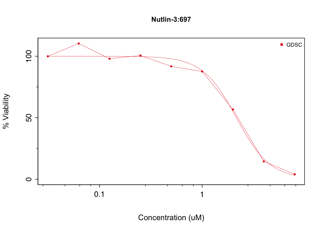
And get the sensitivity measure values for all cell lines for Nutlin-3 and Erlotinib:
sens_mat <- summarizeSensitivityProfiles(GDSC, sensitivity.measure = 'ic50_published', drugs = c('Nutlin-3', 'Erlotinib'), verbose = FALSE) %>% t()
sens_mat <- 9-log10(sens_mat)
dim(sens_mat)
## [1] 1124 2Unfortunately there isn’t a convenience function to extract the dose response data itself, but this can be done as follows:
#get the information about the curve of interest
drug_profiles <- GDSC@sensitivity$info %>%
    tibble::rownames_to_column('curve_id') %>%
    dplyr::filter(drugid=='Nutlin-3', cellid=='697')
drug_profiles
## curve_id cellid drugid drug.name nbr.conc.tested min.Dose.uM
## 1 drugid_1047_697 697 Nutlin-3 NUTLIN3A 9 0.03125
## max.Dose.uM duration_h
## 1 8 72#the raw data is stored in a 3D matrix, can extract as follows:
GDSC@sensitivity$raw["drugid_1047_697",,]## Dose Viability
## doses1 "0.03125" "99.9083625051504"
## doses2 "0.0625" "110.360194300232"
## doses3 "0.125" "97.9893987166772"
## doses4 "0.25" "100.571670763227"
## doses5 "0.5" "91.7495404302393"
## doses6 "1" "87.6252737395088"
## doses7 "2" "56.7022780978287"
## doses8 "4" "14.4871092551858"
## doses9 "8" "4.04710864108274"Molecular profile data
Feature names are symbols for the mutation data and a derivation of ensembl id’s for expression data. Gene name information can be obtained using EnsDb.Hsapiens.v75 package
gene_info <- ensembldb::genes(EnsDb.Hsapiens.v75, filter=GenenameFilter(c('TP53', 'EGFR')), return.type='data.frame') %>%
    dplyr::select(gene_id, gene_name) %>%
    dplyr::mutate(probe_id=paste0(gene_id, '_at'))
gene_info
## gene_id gene_name probe_id
## 1 ENSG00000141510 TP53 ENSG00000141510_at
## 2 ENSG00000146648 EGFR ENSG00000146648_atGet the mutatation and expression data for TP53 and EGFR:
genetic_mat <- summarizeMolecularProfiles(GDSC, mDataType = 'mutation', features = gene_info$gene_name, summary.stat='and', verbose=FALSE) %>% exprs() %>% t()
dim(genetic_mat)
## [1] 1124 2affy_mat <- summarizeMolecularProfiles(GDSC, mDataType = 'rna', features = gene_info$probe_id, summary.stat='first', verbose=FALSE) %>% exprs() %>% t()
dim(affy_mat)## [1] 1124 2Note that I have a half written package called tidyMultiAssay that is available on github which provides convenience functions for the extraction of data from PharmacoSet objects.
Integrated data analysis
Combine data together and turn into a data frame
#sensitivity data
sens_df <- sens_mat %>% as.data.frame() %>% tibble::rownames_to_column('cell_line')

#mutation data
colnames(genetic_mat) <- paste0(colnames(genetic_mat), '_mut' )
genetic_df <- genetic_mat %>% as.data.frame() %>% tibble::rownames_to_column('cell_line')

#affymetrix data
colnames(affy_mat) <- paste0(colnames(affy_mat), '_affy' )
affy_df <- affy_mat %>% as.data.frame() %>% tibble::rownames_to_column('cell_line')

#combine into a single data frame
combined_df <- sens_df %>%
    inner_join(genetic_df, by='cell_line') %>%
    inner_join(affy_df, by='cell_line')

combined_df %>% tbl_df()
## # A tibble: 1,124 x 7
## cell_line `Nutlin-3` Erlotinib TP53_mut EGFR_mut
## <chr> <dbl> <dbl> <fctr> <fctr>
## 1 22RV1 7.892590 NA 1 0
## 2 23132-87 7.680031 NA 0 0
## 3 380 NA NA <NA> <NA>
## 4 5637 6.214938 NA 1 0
## 5 639-V 7.358565 NA 1 0
## 6 647-V 6.072949 NA 1 0
## 7 697 8.694393 8.576254 0 0
## 8 769-P 7.176188 NA 0 0
## 9 786-0 6.995861 NA 1 0
## 10 8305C 6.225848 NA 1 0
## # ... with 1,114 more rows, and 2 more variables:
## # ENSG00000141510_at_affy <dbl>, ENSG00000146648_at_affy <dbl>Now do some basic modelling. Nutlin-3 is more effective in TP53 wild type than mutant cell lines:
lm(`Nutlin-3`~TP53_mut, data=combined_df) %>% summary()##
## Call:
## lm(formula = `Nutlin-3` ~ TP53_mut, data = combined_df)
##
## Residuals:
## Min 1Q Median 3Q Max
## -1.84317 -0.45086 -0.04256 0.46663 2.12744
##
## Coefficients:
## Estimate Std. Error t value Pr(>|t|)
## (Intercept) 7.69481 0.04444 173.16 <2e-16 ***
## TP53_mut1 -1.07415 0.05490 -19.56 <2e-16 ***
## ---
## Signif. codes: 0 '***' 0.001 '**' 0.01 '*' 0.05 '.' 0.1 ' ' 1
##
## Residual standard error: 0.671 on 659 degrees of freedom
## (463 observations deleted due to missingness)
## Multiple R-squared: 0.3674, Adjusted R-squared: 0.3665
## F-statistic: 382.8 on 1 and 659 DF, p-value: < 2.2e-16ggplot(combined_df, aes(y=`Nutlin-3`, x=TP53_mut)) + geom_violin() + geom_point()## Warning: Removed 463 rows containing non-finite values (stat_ydensity).## Warning: Removed 463 rows containing missing values (geom_point).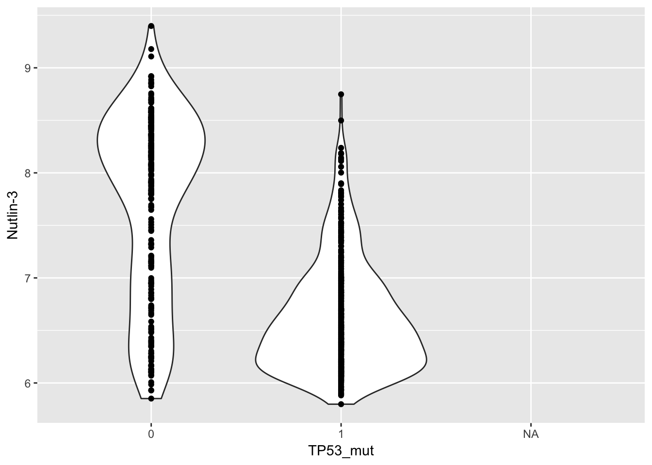
Whereas Erlotinib is more effective in cell lines with high levels of expression of its target, EGFR.
lm(Erlotinib~ENSG00000146648_at_affy, data=combined_df) %>% summary()##
## Call:
## lm(formula = Erlotinib ~ ENSG00000146648_at_affy, data = combined_df)
##
## Residuals:
## Min 1Q Median 3Q Max
## -2.1594 -0.4591 -0.1275 0.3527 3.1857
##
## Coefficients:
## Estimate Std. Error t value Pr(>|t|)
## (Intercept) 4.99793 0.28864 17.315 < 2e-16 ***
## ENSG00000146648_at_affy 0.38049 0.05188 7.335 2.32e-12 ***
## ---
## Signif. codes: 0 '***' 0.001 '**' 0.01 '*' 0.05 '.' 0.1 ' ' 1
##
## Residual standard error: 0.6671 on 285 degrees of freedom
## (837 observations deleted due to missingness)
## Multiple R-squared: 0.1588, Adjusted R-squared: 0.1558
## F-statistic: 53.8 on 1 and 285 DF, p-value: 2.319e-12ggplot(combined_df, aes(y=Erlotinib, x=ENSG00000146648_at_affy)) + geom_point() + geom_smooth(method='lm')## Warning: Removed 837 rows containing non-finite values (stat_smooth).## Warning: Removed 837 rows containing missing values (geom_point).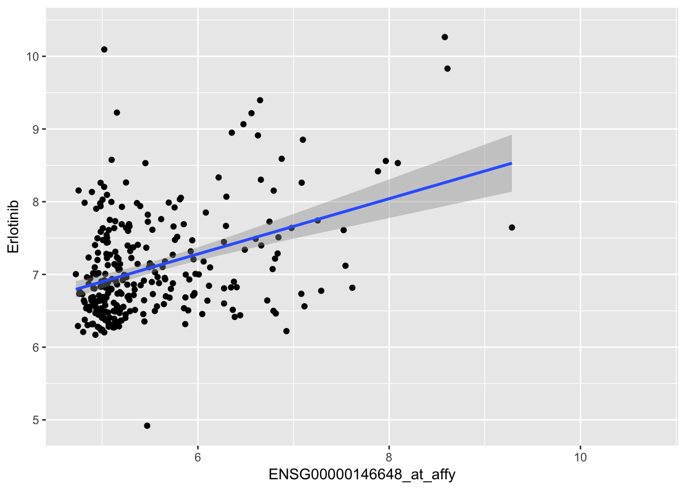
The extension of this is to treat tissue as a covariate since some tissues have higher expression than others or have a higher level of mutation.
The Bayesian bit
There are several sources of uncertainty that are not accounted for by using a simple linear model:
- How accurate is the sensitivity measure estimate and how much information are we losing by converting the dose response curve to a single value?
- Are we able to measure resistant and sensitive cell lines equally accurately?
- How accurate is our classifcation of mutation status - might we have missed mutations in some cell lines, and erroneously called variants in others? How sure can we be of the functional signifance of a mutation?
Could a Bayesian framework allow us to calculate a posterior distribution of effect size of a genetic feature on response to compound?
Session Info
sessionInfo()## R version 3.4.0 (2017-04-21)
## Platform: x86_64-apple-darwin15.6.0 (64-bit)
## Running under: macOS Sierra 10.12.6
##
## Matrix products: default
## BLAS: /Library/Frameworks/R.framework/Versions/3.4/Resources/lib/libRblas.0.dylib
## LAPACK: /Library/Frameworks/R.framework/Versions/3.4/Resources/lib/libRlapack.dylib
##
## locale:
## [1] en_GB.UTF-8/en_GB.UTF-8/en_GB.UTF-8/C/en_GB.UTF-8/en_GB.UTF-8
##
## attached base packages:
## [1] stats4 parallel methods stats graphics grDevices utils
## [8] datasets base
##
## other attached packages:
## [1] bindrcpp_0.2 EnsDb.Hsapiens.v75_2.1.0
## [3] ensembldb_2.0.4 AnnotationFilter_1.0.0
## [5] GenomicFeatures_1.28.5 AnnotationDbi_1.38.2
## [7] GenomicRanges_1.28.6 GenomeInfoDb_1.12.3
## [9] IRanges_2.10.5 S4Vectors_0.14.7
## [11] ggplot2_2.2.1 Biobase_2.36.2
## [13] BiocGenerics_0.22.1 dplyr_0.7.4
## [15] PharmacoGx_1.6.1
##
## loaded via a namespace (and not attached):
## [1] lsa_0.73.1 ProtGenerics_1.8.0
## [3] bitops_1.0-6 matrixStats_0.52.2
## [5] bit64_0.9-7 httr_1.3.1
## [7] RColorBrewer_1.1-2 rprojroot_1.2
## [9] SnowballC_0.5.1 tools_3.4.0
## [11] backports_1.1.1 R6_2.2.2
## [13] KernSmooth_2.23-15 sm_2.2-5.4
## [15] DBI_0.7 lazyeval_0.2.1
## [17] colorspace_1.3-2 gridExtra_2.3
## [19] curl_3.0 bit_1.1-12
## [21] compiler_3.4.0 DelayedArray_0.2.7
## [23] labeling_0.3 rtracklayer_1.36.6
## [25] bookdown_0.5 slam_0.1-40
## [27] caTools_1.17.1 scales_0.5.0
## [29] relations_0.6-7 quadprog_1.5-5
## [31] stringr_1.2.0 digest_0.6.12
## [33] Rsamtools_1.28.0 rmarkdown_1.6
## [35] XVector_0.16.0 pkgconfig_2.0.1
## [37] htmltools_0.3.6 plotrix_3.6-6
## [39] limma_3.32.10 maps_3.2.0
## [41] rlang_0.1.6 RSQLite_2.0
## [43] BiocInstaller_1.26.1 shiny_1.0.5
## [45] bindr_0.1 BiocParallel_1.10.1
## [47] gtools_3.5.0 RCurl_1.95-4.8
## [49] magrittr_1.5 GenomeInfoDbData_0.99.0
## [51] Matrix_1.2-11 Rcpp_0.12.14
## [53] celestial_1.4.1 munsell_0.4.3
## [55] piano_1.16.4 stringi_1.1.5
## [57] yaml_2.1.16 MASS_7.3-47
## [59] SummarizedExperiment_1.6.5 zlibbioc_1.22.0
## [61] AnnotationHub_2.8.3 gplots_3.0.1
## [63] plyr_1.8.4 grid_3.4.0
## [65] blob_1.1.0 gdata_2.18.0
## [67] lattice_0.20-35 Biostrings_2.44.2
## [69] mapproj_1.2-5 knitr_1.17
## [71] fgsea_1.2.1 igraph_1.1.2
## [73] reshape2_1.4.2 marray_1.54.0
## [75] biomaRt_2.32.1 fastmatch_1.1-0
## [77] NISTunits_1.0.1 XML_3.98-1.9
## [79] glue_1.2.0 evaluate_0.10.1
## [81] blogdown_0.2 downloader_0.4
## [83] data.table_1.10.4-3 httpuv_1.3.5
## [85] gtable_0.2.0 RANN_2.5.1
## [87] assertthat_0.2.0 mime_0.5
## [89] xtable_1.8-2 pracma_2.0.7
## [91] tibble_1.3.4 GenomicAlignments_1.12.2
## [93] memoise_1.1.0 sets_1.0-17
## [95] cluster_2.0.6 interactiveDisplayBase_1.14.0
## [97] magicaxis_2.0.3